
Table of Contents
Aggregate data is a cornerstone of modern data analytics, providing a means to distill vast quantities of information into meaningful patterns and insights. This guide delves into the world of aggregate queries, exploring their crucial role in data analytics, the techniques for effective data summarization, and the advanced methods for data aggregation. It also offers practical advice on using R for aggregate data manipulation and expands the toolkit with R’s powerful aggregate functions. With a focus on practical application and efficiency, this guide is an essential resource for anyone looking to master the art of uncovering patterns through aggregate data.
Key Takeaways
- Aggregate queries are foundational in data analytics, enabling the extraction of significant patterns and insights from large datasets.
- Effective data summarization techniques, such as comparative analysis and robust data insights with R’s fivenum(), are critical for insightful statistical analysis.
- Advanced methods, including indexing aggregate queries and polynomial batch coding, offer efficient retrieval and new opportunities in data analysis.
- Practical guides for using R to aggregate daily data, implement rolling averages, and add index columns empower users to handle time series and data manipulation with proficiency.
- R’s aggregate functions, including the apply family and xtabs(), are versatile tools that enhance data organization and sampling, essential for comprehensive data analysis.
Understanding Aggregate Queries and Their Importance in Data Analytics

Defining Aggregate Queries and Their Functions
Aggregate queries are pivotal in the realm of data analytics, serving as the backbone for summarizing and extracting valuable insights from large datasets. They enable the computation of summary statistics such as SUM, COUNT, MIN/MAX, and MEAN. These queries are designed to process data in a collective manner, which allows for a more efficient analysis compared to examining individual records.
Aggregate queries function by grouping data based on specific criteria and then applying aggregate functions to these groups. The following table illustrates some common aggregate functions and their purposes:
| Function | Purpose |
|---|---|
| SUM | Totals the values in a column |
| COUNT | Counts the number of non-null entries |
| MIN/MAX | Finds the minimum/maximum value |
| MEAN | Calculates the average value |
Aggregate queries not only simplify the data but also enhance the performance of data retrieval by reducing the amount of data that needs to be processed.
Despite their utility, constructing an effective aggregate query requires careful consideration of the data structure and the specific insights sought. The choice of index and the design of the query can significantly impact the efficiency and accuracy of the results obtained.
The Role of Aggregate Queries in Modern Data Analysis
In the realm of modern data analysis, aggregate queries are indispensable tools for synthesizing and interpreting vast amounts of information. They enable analysts to distill complex datasets into meaningful summaries, providing insights that drive strategic decision-making.
Aggregate queries serve as the backbone for a variety of analytical tasks, from generating reports to informing policy decisions. Their ability to quickly process and summarize data makes them particularly valuable in environments where time and accuracy are of the essence.
The versatility of aggregate queries allows for a wide range of applications, adapting to the ever-evolving landscape of data analytics.
Despite their utility, aggregate queries also present challenges. The complexity of data structures and the need for expressive querying mechanisms often require advanced techniques and tools. As data analytics continues to grow in sophistication, the development of more robust aggregate query protocols remains a critical area of research and innovation.
Challenges and Opportunities in Aggregate Data Querying
Aggregate data querying is a cornerstone of data analytics, yet it faces significant challenges. The complexity and variety of aggregate queries often exceed the capabilities of existing protocols, leading to limitations in expressiveness and performance. For instance, many systems struggle with keyword-based expressive queries and are unable to support a wide range of aggregate functions.
Despite these challenges, there are substantial opportunities for innovation in this space. Fast query response times and the assurance of privacy in aggregate queries are just the beginning. The development of new techniques that can handle complex operations, such as various JOINs, using advanced batch coding and indexing schemes, is a promising research direction.
The pursuit of efficient and private aggregate querying mechanisms is not just a technical challenge but a gateway to unlocking the full potential of data analytics.
The table below highlights the current limitations and potential advancements in aggregate data querying:
| Current Limitations | Potential Advancements |
|---|---|
| Limited expressiveness for complex queries | Development of expressive querying mechanisms |
| Privacy concerns in data querying | Implementation of privacy-preserving protocols |
| Inefficiency in handling diverse aggregations | Exploration of batch coding and indexing schemes |
Techniques for Effective Data Summarization

Comparative Analysis: tapply() vs. group_by() and summarize()
In the realm of R programming, data summarization is a pivotal task that often involves the use of aggregate functions. The choice between tapply() and the group_by() followed by summarize() combo from the dplyr package can significantly influence the efficiency and readability of your code.
When dealing with complex data sets, tapply() is typically used in base R for applying a function over subsets of a vector. It is particularly useful for concise operations on categorized data. On the other hand, group_by() and summarize() offer a more intuitive syntax and additional flexibility, especially when working with data frames and multiple grouping variables.
Here’s a quick comparison of their usage:
tapply(): Best for simple, quick operations on arrays or matrices.group_by()andsummarize(): Ideal for detailed data frame manipulations and when dealing with multiple grouping variables.
While tapply() might be more straightforward for quick, one-off calculations, group_by() and summarize() provide a more robust framework for complex data manipulation tasks, allowing for a clearer expression of data analysis intentions.
Utilizing R’s fivenum() for Robust Data Insights
R’s fivenum() function is a powerful tool for statisticians and data analysts. It provides a five-number summary of a dataset, which includes the minimum, lower-hinge, median, upper-hinge, and maximum. This summary is essential for understanding the distribution of data without getting lost in the noise of every single data point.
The use of fivenum() can significantly streamline the exploratory data analysis process, offering a quick snapshot of data distribution that can guide further analysis. For instance, consider a dataset of annual sales figures for a retail company. The five-number summary could look like this:
| Year | Minimum | Lower-Hinge | Median | Upper-Hinge | Maximum |
|---|---|---|---|---|---|
| 2021 | $10,000 | $25,000 | $50,000 | $75,000 | $100,000 |
| 2022 | $15,000 | $30,000 | $55,000 | $80,000 | $110,000 |
By identifying outliers and understanding the spread of the data, analysts can make more informed decisions and provide more accurate forecasts.
When working with fivenum(), it’s important to remember that it is just one part of a comprehensive data analysis toolkit. While it provides a quick and useful summary, it should be complemented with other methods to fully uncover the patterns and insights within the data.
Mastering Grouped Counting and Data Visualization in R
In the realm of R programming, grouped counting is a pivotal technique for summarizing categorical data. It allows analysts to quickly ascertain the frequency of categories within a dataset, providing a foundation for more complex analysis. For instance, using the dplyr package, one can effortlessly count the occurrences of a category with the group_by() and summarize() functions.
Effective data visualization in R often follows grouped counting. It translates the numerical insights into graphical representations that are easier to interpret and share. Libraries such as ggplot2 enable the creation of compelling visualizations, from scatter plots that reveal relationships between variables to histograms that display data distributions.
By mastering these skills, analysts can deliver powerful stories told through data, making the invisible patterns visible to decision-makers.
Here’s an example of how grouped counting might look in a dataset of sales by region:
| Region | Sales Count |
|---|---|
| North | 120 |
| South | 95 |
| East | 78 |
| West | 104 |
To further enhance the analysis, one might consider creating a bar chart to visually compare the sales count across regions, thus making the data more accessible and actionable.
Advanced Methods for Data Aggregation

Indexing Aggregate Queries for Efficient Retrieval
Efficient data retrieval is paramount in data analytics, and indexing aggregate queries plays a crucial role in this process. By creating indexes tailored to specific aggregate queries, analysts can significantly reduce the time it takes to fetch and compute results from large datasets. This approach is particularly beneficial for operations like SUM, COUNT, MIN/MAX, and MEAN, which are frequently used in data analysis.
Indexes of aggregate queries enable the batching of multiple requests, streamlining the interaction with the database. This not only improves performance but also simplifies the user experience, as the complexity of the underlying database structure is abstracted away.
The following table illustrates the types of queries supported by an indexed aggregate query framework:
| Query Type | Description |
|---|---|
| SUM | Totals the values of a specified column |
| COUNT | Counts the number of non-null entries |
| MIN/MAX | Finds the minimum or maximum value |
| MEAN | Calculates the average value |
Creating an effective index involves understanding the data structure and the queries that will be run against it. The process typically includes identifying the most common queries and structuring the index to optimize for those operations. As a result, the retrieval of aggregate data becomes a more efficient and streamlined process.
Exploring Polynomial Batch Coding and Its Applications
Polynomial batch coding represents a significant advancement in the realm of data storage and retrieval. By modifying the vector-matrix model, Henry’s approach allows for the creation of encoded buckets that are typically smaller than the original database. This results in reduced costs for hosting, communication, and computation.
The applications of polynomial batch coding extend to enhancing data security and efficiency. For instance, the use of indexes of batch queries enables the aggregation of multiple data blocks through a single request. This not only streamlines the process but also adds a layer of security, as every user query must pass through the same batch index, minimizing the risk of information leakage.
The integration of u-ary coding with polynomial batch coding further optimizes the handling of multiple user queries, transforming them into a single query vector. The servers’ responses to these batched queries maintain the integrity of the data while ensuring efficient retrieval.
The table below illustrates the impact of polynomial batch coding on server load and query processing time:
| Metric | Without Coding | With Polynomial Batch Coding |
|---|---|---|
| Server Load (GB) | 100 | 75 |
| Query Processing Time (s) | 30 | 20 |
By adopting polynomial batch coding, organizations can achieve a more cost-effective and secure data management system.
Leveraging Standard Aggregate Vectors for Enhanced Analysis
The concept of standard aggregate vectors plays a pivotal role in the realm of data aggregation. These vectors, when applied to databases, facilitate component-wise aggregation, which is essential for summarizing and analyzing large datasets efficiently. By utilizing standard aggregate vectors, analysts can transform complex data into a more manageable form, making it easier to uncover patterns and insights.
In the context of secure data querying, standard aggregate vectors have been instrumental in enabling users to submit aggregate statistical queries on untrusted databases with provable security guarantees. This advancement is particularly significant as it ensures the privacy of sensitive information while still allowing for comprehensive data analysis.
The integration of standard aggregate vectors with polynomial batch coding techniques has expanded the capabilities of aggregate queries. This synergy not only enhances the efficiency of data retrieval but also broadens the scope of potential searches, offering new opportunities for in-depth data exploration.
For example, consider the following table that outlines the relationship between the number of values in a filter clause and the dimensionality of the query vector:
| Filter Clause Values | Query Vector Dimension |
|---|---|
| 10 | 10-dimensional |
| 50 | 50-dimensional |
| 100 | 100-dimensional |
This table illustrates how the dimensionality of the query vector scales with the number of possible values for a variable in the filter clause, which is a fundamental aspect of constructing efficient aggregate queries.
Practical Guides to Aggregate Data in R

Aggregating Daily Data to Months and Years
When working with time series data, the granularity of daily records often requires aggregation for meaningful analysis. Aggregating daily data to months and years allows for trend identification and seasonal pattern analysis, which are crucial for strategic decision-making. In R, this can be achieved using various packages and functions, such as xts, lubridate, or even base R functions.
To aggregate data effectively, one must follow a series of steps:
- Convert the data into a date format recognized by R.
- Use appropriate functions to group data by desired time frames.
- Summarize the data within these groups to extract insights.
Aggregating data not only simplifies the dataset but also enhances the clarity of the insights derived from it.
It’s important to note that while aggregation simplifies data, it may also lead to the loss of detail. Therefore, it’s essential to balance the need for simplicity with the requirement to maintain sufficient detail for analysis.
Implementing Rolling Averages for Time Series Analysis
Rolling averages, also known as moving averages, are essential for smoothing time series data to identify trends. Implementing rolling averages in R is straightforward, thanks to functions like rollapply from the zoo package. This function allows for the application of any function, such as mean, median, or sum, over a rolling window of observations.
To calculate a simple moving average, you can use the rollmean function from the zoo package or the rollify function from the tidyquant package for a tidyverse approach. Here’s a basic example using rollmean:
library(zoo)
rolling_avg <- rollmean(your_data, k, fill = NA)
Where your_data is your time series data and k is the size of the moving window.
Remember, the choice of window size k can significantly affect the analysis. A smaller k retains more variability, while a larger k provides a smoother trend.
For more complex analyses, such as rolling correlation, the rollapply function is versatile and powerful. It can handle varying window sizes and even custom functions for in-depth time series analysis.
Adding Index Columns to Data Frames for Better Manipulation
In the pursuit of efficient data analysis, adding index columns to data frames can significantly streamline the manipulation process. This technique allows for quicker sorting, subsetting, and grouping operations, which are essential in handling large datasets.
To add an index column in R, one can utilize the row_number() function from the dplyr package, or simply assign a sequence of numbers to a new column. Here’s a concise example:
df$index <- 1:nrow(df)
By assigning an index, you create a unique identifier for each row, which can be invaluable for tracking changes and ensuring data integrity during complex transformations.
Remember, while an index column facilitates data manipulation, it should be used judiciously to avoid redundancy and maintain database normalization principles. When working with time series data, for instance, consider whether the timestamp can serve as a natural index before adding a separate one.
Expanding Your Toolkit with R’s Aggregate Functions
Navigating the Apply Family: apply(), lapply(), sapply(), and tapply()
The ‘apply’ family of functions in R is a cornerstone for efficient data manipulation and analysis. apply() is used for applying a function to the rows or columns of a matrix. In contrast, lapply() and sapply() are designed for lists and vectors, returning a list and a simplified version, respectively. tapply() is particularly useful for applying a function over subsets of a vector.
- apply(): Matrix application
- lapply(): List application, returns list
- sapply(): List application, returns simplified structure
- tapply(): Subset application
Mastering these functions can significantly enhance your data analysis workflow, allowing for more concise and readable code.
Understanding when and how to use each function is crucial for any data analyst working with R. While apply() is often used for its simplicity in iterating over matrix dimensions, lapply() and sapply() provide a more functional approach to list operations. tapply() shines when you need to break down a complex vector into manageable groups and perform calculations on each subset.
Harnessing the Power of Sampling with sample()
The sample() function in R is a cornerstone for simulating randomness and conducting probabilistic analyses. It enables the selection of random samples from a dataset, ensuring that each subset is representative of the larger population. This function is particularly useful for tasks such as bootstrapping, Monte Carlo simulations, and creating training and test sets for machine learning models.
The versatility of sample() extends beyond simple random sampling. It can handle weighted sampling, allowing for more complex probabilistic models that account for varying probabilities of selection.
When using sample(), it’s important to set a seed for reproducibility, especially when sharing code or conducting experiments that require consistent results. Below is a list of common parameters and their descriptions:
x: The original vector or dataset from which to sample.size: The number of items to sample.replace: Whether sampling should be done with replacement.prob: A vector of probability weights for each element inx.
Understanding and utilizing the sample() function can significantly enhance the analytical capabilities of any data scientist or statistician working with R.
Organizing Data with xtabs() for Clearer Insights
The xtabs() function in R is a powerful tool for creating contingency tables, which are essential for organizing categorical data. By structuring data into a tabular format, xtabs() facilitates a clearer understanding of the relationships between variables. It’s particularly useful when dealing with large datasets where patterns might not be immediately obvious.
When using xtabs(), it’s important to follow a few steps:
- Identify the variables you want to cross-tabulate.
- Determine the function’s formula interface, which typically follows the
xtabs(data ~ var1 + var2)format. - Execute the function and interpret the resulting table.
The simplicity of xtabs() belies its utility in exploratory data analysis, making it an indispensable part of the data analyst’s toolkit.
For example, consider a dataset with two categorical variables, Gender and Preference. An xtabs() output might look like this:
| Gender | Tea | Coffee |
|---|---|---|
| Male | 120 | 135 |
| Female | 130 | 125 |
This table quickly reveals the distribution of preferences across genders, highlighting the ease with which xtabs() can bring data to life.
Conclusion
Throughout this guide, we have explored the multifaceted world of aggregate data, uncovering the patterns and techniques that enable effective data analysis. From the innovative frameworks that enhance IT-PIR protocols to the practical applications in R programming, we’ve seen how aggregate queries are pivotal in extracting meaningful insights from vast datasets. The development of indexes for aggregate queries, such as SUM, COUNT, MEAN, and Histogram, has revolutionized the way we interact with data, allowing for more efficient and private data retrieval. As we continue to push the boundaries of data analytics, the knowledge and strategies discussed here will serve as a cornerstone for professionals and enthusiasts alike, empowering them to harness the full potential of aggregate data in their respective fields.
Frequently Asked Questions
What are aggregate queries and why are they important in data analytics?
Aggregate queries are database queries that perform calculations on a set of values to return a single value, such as SUM, COUNT, or MEAN. They are crucial in data analytics for summarizing data, identifying trends, and supporting decision-making processes.
How do Splinter and other protocols improve the privacy of aggregate queries?
Protocols like Splinter aim to privatize aggregate queries by hiding sensitive parameters in a user’s query. This enhances the security of data analytics by protecting user privacy while still allowing for the extraction of valuable insights.
What is polynomial batch coding and how does it relate to data aggregation?
Polynomial batch coding is a technique used to encode data in a way that supports efficient retrieval of aggregate information. It augments IT-PIR protocols with aggregate queries, enabling new opportunities for data analysis.
How can indexes of aggregate queries improve data retrieval?
Indexes of aggregate queries allow for the efficient retrieval of results for common aggregate queries like SUM, COUNT, and MEAN with a single interaction with the database, streamlining the data aggregation process.
What are the benefits of using R’s apply family of functions for data aggregation?
R’s apply family of functions, including apply(), lapply(), sapply(), and tapply(), provide a versatile set of tools for applying functions to data structures in R. They help in simplifying code, improving readability, and ensuring efficient data manipulation and aggregation.
How does the sample() function in R aid in data analysis?
The sample() function in R is used for sampling data, which is a fundamental technique in data analysis. It allows analysts to select a representative subset of data for examination, which can be useful for making inferences about larger datasets.